[논문리뷰] Temporal Fusion Transformers for Interpretable Multi-horizon Time Series Forecasting (2/3)
4. Model Architecture
우리는 TFT를 설계하여 각 input type에 대한 feature representation을 구축하고 다양한 문제에 대해 높은 forecasting performance를 제공한다. TFT의 구조를 그림으로 그리면 Fig. 2와 같다.

4.1. Gating Mechanisms
Exogenous Input과 Target 사이의 관계는 미리 알 수 없어 어떠한 변수들이 연관되어 있는지 예측하기 어렵게 한다. 또한 필요한 non-linear processing의 길이를 결정하기 힘들며 단순한 모델들이 훨씬 효과적일 수 있는 small or noisy dataset이 존재하기도 한다. TFT는 필요할 때만 non-linear processing을 하여 모델의 유연성을 높이고자 Gated Residual Network (GRN)을 제안한다. GRN은 초기 입력 $\mathbf{a}$와 optional context vector $\mathbf{c}$를 받아 다음과 같이 처리한다.
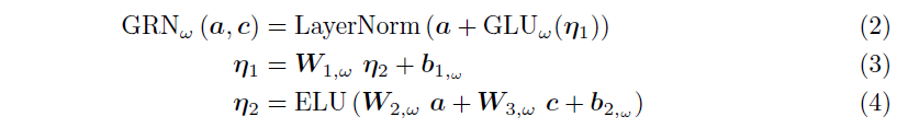
여기서 ELU는 Exponential Linear Unit Activation Function을 의미하고, $\eta_1, \eta_2 \in \mathbb{R}^{d_{model}}$은 모두 intermediate layer에 해당하며, LayerNorm은 standard layer normalization, $\omega$는 weight sharing index를 의미한다. ELU는 입력값이 0보다 크면 Identify Function으로 동작하며, 0보다 매우 작을 때는 constant output을 생성한다. 이후 Gated Linear Unit (GLU)을 사용하여 주어진 데이터셋에서 필요하지 않은 부분을 제거한다. GLU의 수식은 다음과 같다.

이때 $\sigma(\cdot)$는 sigmoid activation function, $\gamma \in \mathbb{R}^{d_{model}}$은 input, $\mathbf{W}_{(\cdot)} \in \mathbb{R}^{d_{model} \times d_{model}}$과 $\mathbf{b}_{(\cdot)} \in \mathbb{R}^{d_{model}}$은 weight와 bias를 의미한다. $\odot$은 element-wise Hadamard product이고, $d_{model}$은 hidden state의 크기이다. 전체적인 GRN의 모습을 그림으로 표현하면 다음과 같다.

4.2. Variable Selection Networks
여러 변수를 사용할 수 있지만, 각 변수가 출력에 대해 얼만큼의 기여도를 갖는지는 알 수 없다. TFT는 variable selection network를 사용하여 static covariate와 time-dependent covariate 모두에 대해 instance-wise 변수 선택을 제공하도록 설계되었다. 변수 선택은 prediction problem에 가장 중요한 변수를 파악하는 데 도움을 주는 것뿐만 아니라, 모델의 성능에 악영향을 미칠 수 있는 불필요한 noisy input을 제거하여 TFT의 성능을 향상시키는 효과를 준다. 대부분의 time series 데이터셋에는 less predictive content가 포함되어 있으므로, 변수 선택을 통해 학습 능력을 가장 중요한 특성에만 집중시킴으로써 모델 성능을 크게 향상시킬 수 있다.
우리는 categorical variable에 대해 entity embedding을 사용하여 feature representation을 생성하며, continuous variable에 대해서는 linear transformation을 사용한다. 이로써 각 입력 변수를 $d_{model}$ 차원의 벡터로 변환하고, 이를 다음 layer와 일치하는 차원으로 맞춘다. static, past, future input은 각각 별개의 variable selection network를 사용한다. 일반성을 잃지 않고, past input에 대한 variable selection network를 보자.
$\xi_t^{(j)} \in \mathbb{R}^{d_{model}}$이 time $t$에서 $j$번째 variable의 transformed input이라 하고, $\Xi_t=\Big[ \xi_t^{(1)^T}, \cdots, \xi_t^{(m_\chi)^T} \Big]^T$를 time $t$의 모든 past input을 flatten한 벡터라 하자. 이때 variable selection weight는 $\Xi_t$와 external context vector $\mathbf{c}_s$를 GRN과 softmax layer를 거쳐 나온 값으로, 다음과 같이 구해진다.

이렇게 얻어진 $\mathbf{v}_{\chi_t} \in \mathbb{R}^{m_\chi}$는 variable selection weight를 나타내는 벡터이고, $\mathbf{c}_s$는 static covariate encoder를 통해 얻을 수 있다. static variable에 대해서는 context vector $\mathbf{c}_s$가 생략된다. 또한, 각 time step에서 $\xi_t^{(j)}$에는 다음과 같이 GRN이 적용된다.

이렇게 얻어진 $\widetilde{\xi}_t^{(j)}$는 variable $j$에 대한 processed feature vector이다. 각 variable은 모든 time step $t$에 적응되는 고유의 $GRN_{\xi(j)}$를 갖게 된다. 이렇게 얻어진 processed feature를 앞에서 구한 variable selection weight과 결합하면 다음의 식을 얻을 수 있다.

이때 $v_{\chi_t}^{(j)}$는 $\mathbf{v}_{\chi_t}$의 $j$-th element를 뜻한다. Variable Selection Network의 전체적인 과정을 그림으로 표현하면 다음과 같다.

4.3. Static Covariate Encoders
다른 time series forecasting architecture와는 달리, TFT는 static metadata로부터 정보를 통합하도록 설계되었다. TFT에서는 별도의 GRN 인코더를 사용하여 네 가지의 context vector $\mathbf{c}_s$, $\mathbf{c}_e$, $\mathbf{c}_c$, $\mathbf{c}_h$를 생성하는데, 이러한 context vector는 temporal fusion decoder에서 사용된다. 각각의 역할은 (1) temporal variable selection ($\mathbf{c}_s$), (2) local processing of temporal feature ($\mathbf{c}_c$, $\mathbf{c}_h$), 그리고 (3) static information에 대한 temporal feature ($\mathbf{c}_e$)이다. 예를 들어, $\zeta$가 static variable selection network의 output이라면 temporal variable selection을 위한 context는 $\mathbf{c}_s = GRN_{\mathbf{c}_s}(\zeta)$와 같이 인코딩될 것이다.
4.4. Interpretable Multi-Head Attention
TFT는 Self-Attention Mechanism을 통해 다른 시점에 대한 Long-Term Relation을 파악하는데, 우리는 Transformer 기반의 Multi-Head Attention을 통해 explainability를 강화시켰다. 일반적으로 Attention Mechanism의 Attention은 다음과 같이 계산된다.

이때 $\mathbf{V} \in \mathbb{R}^{N \times d_V}$는 scale value, $\mathbf{K}, \mathbf{Q} \in \mathbb{R}^{N \times d_{attn}}$는 각각 key와 query를 뜻하고 $A$는 normalization function이다. $A$의 식은 일반적으로 다음과 같이 정의된다.

기본적인 Attention의 Learning Capacity를 개선하기 위해서 Multi-Head Attention을 제안하였으며, 이는 여러 Head에서 각기 다른 Representation Subspace를 사용함으로써 학습 효용성을 개선하는 방식이라고 볼 수 있다.

이때 $\mathbf{W}_K^{(h)} \in \mathbb{R}^{d_{model} \times d_{attn}}$, $\mathbf{W}_Q^{(h)} \in \mathbb{R}^{d_{model} \times d_{attn}}$, $\mathbf{W}_V^{(h)} \in \mathbb{R}^{d_{model} \times d_V}$는 각각 head-specific weights for keys, queries, and values이고, $\mathbf{W}_H \in \mathbb{R}^{(m_H \cdot d_V) \times d_{model}}$은 $\mathbf{H}_h$를 나열한 값을 선형적으로 결합해주는 역할을 한다. 다른 값들이 각각 다른 Head에서 사용되기 때문에 Attention의 가중치가 단독으로는 특정 Feature의 중요성을 나타내는 지표가 되기 어려운데, 따라서 다음과 같이 Multi-Head Attention을 수정하여 각 Head에서 값을 공유할 수 있도록 만들었다.

각 Head는 다른 시간 Pattern을 학습하고 이들이 입력으로 단순히 Ensemble 된 것이라고 생각할 수 있다. 이 방법은 $A(\mathbf{Q}, \mathbf{K})$와 비교하였을 때 증가된 Representation Capacity를 제공함은 물론, 하나의 Attention Weight Output을 제공함을 통해 Interpretability를 확보할 수 있다.
4.5. Temporal Fusion Decoder
Temporal Fusion Decoder는 데이터셋에 존재하는 시간 간의 관계에 대해 학습한다.
4.5.1. Locality Enhancement with Sequence-to-Sequence Layer
time series 데이터에서는 anomalies, change-points 또는 cyclical pattern과 관련하여 주변 값과 비교하여 중요한 지점을 식별한다. local context를 활용하여 point-wise value의 패턴 정보를 사용하여 기능을 구축함으로써 attention-based 아키텍처의 성능을 향상시킬 수 있다. 그러나 이는 observed input이 있는 경우 past와 future input의 수가 다르기 때문에 적합하지 않을 수 있다. 따라서 우리는 이러한 차이를 처리하기 위해 sequence-to-sequence model을 적용하여 $\widetilde{\xi}_{t-k:t}$를 인코더에 넣고 $\widetilde{\xi}_{t+1:t+\tau_{max}}$를 디코더에 넣는다. 그 결과로 uniform temporal feature이 생성되며, 이는 temporal fusion decoder로의 input으로 사용된다. 이를 position index $n$에 대해 $\phi(t, n) \in \{\phi(t, -k), \cdots, \phi(t, \tau_{max})\}$로 표기할 수 있다.
일반적으로 사용되는 sequence-to-sequence baseline과의 비교를 위해 LSTM encoder-decoder를 사용하지만, 다른 모델도 적용될 수 있다. 이는 또한 input의 시간 순서에 따라 적절한 inductive bias를 제공하기 위해 기본적인 positional encoding을 대체하는 역할도 한다. 또한, static metadata가 local preprocessing에 영향을 미치도록 하기 위해 static covariate encoder로부터 $\mathbf{c}_c$, $\mathbf{c}_h$ context vector를 사용하여 첫 번째 LSTM의 cell state 및 hidden state를 초기화한다. 여기에 gated skip connection을 적용시키는데, position index $n \in [-k, \tau_{max}]$에 대해 식을 쓰면 다음과 같다.

4.5.2. Static Enrichment Layer
Static Covariate는 Temporal Dynamics에서 큰 영향을 미칠 수 있기 때문에 TFT는 Static Enrichment layer를 이용하여 이러한 static metadata의 temporal feature를 강화시킨다. 주어진 position index $n$에 대하여 static enrichment의 식은 다음과 같다.

이때 $GRN_\theta$는 전체 layer에 공유되며, $\mathbf{c}_e$는 static covariate encoder의 context vector이다.
4.5.3. Temporal Self-Attention Layer
이후 모든 static-enriched temporal feature는 $\Theta(t)=[\theta(t, -k), \cdots, \theta(t, \tau)]^T$로 그룹화되고, 다음과 같이 multi-head attention을 적용시킨다.

그 결과 $\mathbf{B}(t)=[\beta(t, -k), \cdots, \beta(t, \tau_{max})]$를 얻을 수 있다. 이렇게 얻어진 값에 대해 각각의 temporal dimension이 그에 해당하는 feature에 상응할 수 있도록 하기 위해 decoder masking을 적용시킨다. Self-Attention Layer는 TFT가 RNN으로는 잡아내기 어려운 long-range dependency를 학습할 수 있도록 해주고, 추가적인 gating layer를 통해 학습을 촉진시킨다. 이를 식으로 적으면 다음과 같다.

4.5.4. Position-wise Feed-forward Layer
이렇게 얻어진 Self-Attention Layer에 추가적인 non-linear processing을 적용한다. Static Enrichment Layer와 유사하게 아래와 같이 GRN을 사용하여 다음의 식을 얻을 수 있다.

전과 마찬가지로 $는 모든 layer에 공유된다. 여기에 gated residual connection을 적용시키고 sequence-to-sequence layer의 결과값을 더해서 LayerNorm을 적용시키면 다음의 식을 얻을 수 있다.

4.6. Quantile Outputs
이러한 과정을 거쳐 최종적으로 TFT는 point forecast의 prediction interval을 생성할 수 있다. Quantile forecast의 식은 다음과 같다.

이때 $\mathbf{W}_q \in \mathbb{R}^{1 \times d}$, $b_q \in \mathbb{R}$은 quantile $q$에 대한 linear coefficient이고, $\tau \in \{1, \cdots, \tau_{max}\}$이다.
5. Loss Functions
TFT는 다음의 quantile loss를 최소화하는 방향으로 학습되었다.

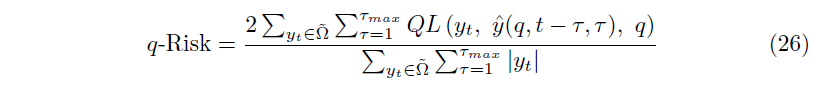
이때 $\Omega$는 $M$개의 sample을 갖는 training data이고, $\mathbf{W}$는 TFT의 weight를 나타낸다. $\mathcal{Q}$는 output quantile의 집합이고, $(\cdot)_+=\max(0, \cdot)$이다. 이 경우 $\widetilde{\Omega}$를 test sample의 집합이라 할 때, normalized quantile loss는 다음과 같이 계산할 수 있다.